myfempy
[TOC]
User’s Guide
This guide introduces the components and commands that define the configuration file required to execute an analysis using MYFEMPY. Depending on the problem setup, adjustments may be necessary; please refer to the help or API documentation for details. Additional Tutorials are provided at the end of this guide.
Presentation
The myfempy project was developed as a finite element solver for multi-physics simulations, intended for academic and research use. Originating from the author’s doctoral thesis, the project has matured into a robust computational framework. Its primary goal is to provide an accessible yet powerful environment for simulation setup and execution, minimizing the need for advanced prior knowledge of numerical methods while maintaining flexibility for expert users.
At its core, myfempy implements a finite element processor that drives the numerical analysis. The workflow is organized into three principal stages:
Pre-processing
- Configuration is performed through API commands.
- Users specify material properties, element types, and boundary conditions.
- Mesh generation is managed via Gmsh, which supplies both geometry and discretization data.
Processing
- The solver core executes finite element computations according to the defined physics and constraints.
- Multi-physics coupling is supported, enabling integration of multiple physical domains within a single simulation.
Post-processing
- Results are exported in formats compatible with visualization tools.
- Output data is structured as VTK files, which can be analyzed and visualized using ParaView.
This architecture emphasizes modularity, extensibility, and interoperability with established open-source tools, positioning myfempy as a versatile platform for computational mechanics and multi-physics research. A typical analysis workflow involves submitting requests (Python dictionaries) through a specific script pattern. The user imports the desired solver, configures the problem by defining materials, finite elements, and geometry, and generates a mesh via Gmsh. Loads and boundary conditions are applied, and the solver computes the solution. Results are exported and visualized in ParaView.
graph LR
U[User] --> MyfempyAPI
MyfempyAPI --> A[Gmsh]
A[Gmsh] --> B[MyfempyCore]
B --> C[Paraview]

style A fill:#006400, stroke:#333, stroke-width:2px
style B fill:#006400, stroke:#333, stroke-width:2px
style C fill:#00008B, stroke:#333, stroke-width:2px
To ensure organized execution, myfempy employs a hierarchical code structure that integrates user requests into a processing pipeline. Input data is validated through controllers in the I/O interface. If commands and data are consistent, they are passed to the solver core, where pre-processing, solution, and post-processing occur. The processed data is then returned through the I/O filters and exported as visualization-ready files (VTK).
graph
  U[InputData] --> B{IO}
  B -->|Yes| C[PreProcess]
  C --> R[CoreSolver]
  R --> D[PostProcess]
  D --> B;
  B -----> O[OutputData]
  B ----->|No| E[ReturnERROR]

style C fill:#006400, stroke:#333, stroke-width:2px
style R fill:#006400, stroke:#333, stroke-width:2px
style D fill:#006400, stroke:#333, stroke-width:2px
style O fill:#00008B, stroke:#333, stroke-width:2px
style E fill:#8B0000,stroke:#333,stroke-width:2px;
How it Works
myfempy is implemented using an object-oriented paradigm, structured around the Bridge design pattern. The system is composed of multiple classes, with user interaction facilitated through APIs that orchestrate the execution of the solver.
The project adopts a black-box architecture: users provide input data, the solver executes the numerical routines, and the system returns output data along with logs for validation.
graph LR
UserInput --> BLACK-BOX
BLACK-BOX --> OutputData
The main API provides direct access to the core components of the project, enabling construction of the Model, definition of Physics, and execution of the Solution.
graph LR
User --> API
API --> Model
API --> Physics
API --> Solve
API --> Results

Model --> Element
Model --> Shape
Model --> Mesh
Model --> Material
Model --> Geometry

Physics --> Loads
Physics --> BoundCond
Physics --> Coupling

Results --> PostProcess

Solve --> Assembler
Solve --> Solver
Pre-Process
API and Solver
# ==============================================================================
# import newAnalysis to set a new problem
# ==============================================================================
from myfempy import newAnalysis
# ==============================================================================
# import a solver to running and analysis the problem set, e.g. SteadyStateLinear
# ==============================================================================
from myfempy import Solver
# ==============================================================================
# now, fea is the API to running the Solver Analysis
# ==============================================================================
fea = newAnalysis(Solver)
Solvers
# ==============================================================================
# currently available solvers for import into the myfempy library
# ==============================================================================
# >see: Table 3 - Solvers List to more informations
# solver options
"SteadyStateLinear"                 # Steady State Linear Solver Class
"SteadyStateLinearIterative"        # Steady State Linear Iterative Solver Class
"DynamicEigenLinear"                # Dynamic Eigen (modal problem) Linear Solver Class
"DynamicHarmonicResponseLinear"     # Dynamic Harmonic Response Forced System Steady State Linear Solver Class

# [adv]
"StaticLinearCyclicSymmPlane"       # Static Linear Cyclic Symmetry Plane Solver Class
"PhononicCrystalInPlane"            # Phononic Crystal In-Plane Solver Class
"HomogenPlane"                      # Homogenization Plane Solver Class
Model
# ==============================================================================
# modeldata is a Python dictionary that contains the commands for model set
# ==============================================================================
modeldata = dict()
Material
# ==============================================================================
# config. material
# ==============================================================================
modeldata["MATERIAL"] = dict()
keys
"MAT":str()		          # material set
      # >see: Table 4 - Material List to more informations
      # options
      'lumped' 			    # lumped material
      'uniaxialstress'	# axial{rod, beams...} behavior material
      'planestress'		  # plane stress behavior
      'planestrain'		  # plane strain behavior
      'solidelastic'		# solid behavior material
      'heatplane'			  # heat behavior material
      'heatsolid'			  # heat behavior material

      # [dev]
      'fluid'

"TYPE":str()			      # material behavior
      # options
      'isotropic'			  # isotropic stress/strain material
      'usermaterial'		# user config. material

"PROPMAT":list[mat_set_1:dict(),..., mat_set_n:dict()] # material properties
      # options
      "NAME": str() 		# material name def
      # isotropic solid parameters
      # >see: Appendix: Table 5 - Consistent Units to more informations
      "EXX": float()		# elasticity modulus in x direction
      "VXY": float() 		# poisson's ratio in x direction
      "GXY": float()		# shear modulus in x direction
      "RHO": float() 		# density of material

      # anisotropic solid parameters
      "EYY": float()
      "VYZ": float()
      "GYZ": float()
      "EZZ": float()
      "VZX": float()
      "GZX": float()

      # heat parameters
      "KXX": float()      # thermal conductivity in x direction
      "KYY": float()      # thermal conductivity in y direction
      "KZZ": float()      # thermal conductivity in z direction
      "CTE": float()      # coefficients thermal expansion

      # [dev] fluid parameters
      "VIS": float()      # viscosity
      "RHO": float() 		  # density of fluid

      # lumped model
      "STIF": float()		  # stiffness lumped
      "DAMP": float()		  # damping lumped

# [adv]
"CLASS": class()          # user new class defined
      #-----------------------
      # example:
      #-----------------------
      # from myfempy import PlaneStress
      # ===============================================================================
      #                    SET NEW MATERIAL <ORTHOTROPIC ELASTIC>
      # ===============================================================================
      # class UserNewMaterial(PlaneStress):
      #     def __init__(self):
      #         super().__init__()
      #     def getMaterialSet():
      #         matset = {
      #             "mat": "planestress",
      #             "type": "orthotropic",
      #         }
      #         return matset
      #     def getElasticTensor(tabmat, inci, element_number, a=None, b=None):
      #         # # material elasticity
      #         EXX = tabmat[int(inci[element_number, 2]) - 1]["EXX"]
      #         EYY = tabmat[int(inci[element_number, 2]) - 1]["EYY"]
      #         # material poisson ratio
      #         VXY = tabmat[int(inci[element_number, 2]) - 1]["VXY"]
      #         VYZ = tabmat[int(inci[element_number, 2]) - 1]["VYZ"]
      #         # EXX = 45E3       # N/mm^2 --> MPa
      #         # EYY = 12E3       # N/mm^2 --> MPa
      #         # VXY = 0.23
      #         # VYX = 0.66
      #         S00 = EXX/(1-VXY*VYZ)
      #         S01 = (VYZ*EXX)/(1-VXY*VYZ)
      #         S10 = (VXY*EYY)/(1-VXY*VYZ)
      #         S11 = EYY/(1-VXY*VYZ)
      #         S22 = (EXX*EYY)/(EXX+EYY+2.0*EYY*VXY)
      #         D = np.zeros((3, 3), dtype=np.float64)
      #         D[0, 0] = S00
      #         D[0, 1] = S01
      #         D[1, 0] = S10
      #         D[1, 1] = S11
      #         D[2, 2] = S22
      #         return D
      #     def getFailureCriteria(stress):
      #         stress
      #         return super().getFailureCriteria()
      # ===============================================================================
Geometry
# ==============================================================================
# config. geometry
# ==============================================================================
modeldata["GEOMETRY"] = dict()
keys
"GEO":str()		      # geometry type
      # options
      'solid' 			      # solid 3D geo.
      'thickness'	        # planes geometries, e.g. plane stress, plates ...
      'frame'		          # rods, beams and frames geometries

"SECTION":str()     # geometry beam cross section set
      # options
      # >see:  Appendix: Cross Section Dimensions to more informations
      'rectangle'
      'rectangle_tube'
      'circle'
      'circle_tube'
      'isection'
      'tsection'
      'csection'
      'lsection'
      'userdefined'

"PROPGEO":list[geo_set_1:dict(),..., geo_set_n:dict()] # geometry properties
      # options
      "NAME": str() 		  # geometry name def

      # parameters defined from the user's cross-section
      "AREACS": float()	# area cross section
      "INERXX":float()	# inercia x diretion
      "INERYY":float()	# inercia y diretion
      "INERZZ":float()	# inercia z diretion
      "THICKN":float()	# thickness of plane/plate

      # user set section dimensions
      # >see: Appendix: Cross Section Dimensions to more informations
      "DIM":dict()		    # dimensional beam cross section
      {
          "b":float()		  # b size
          "h":float()		  # h size
          "t":float()		  # t size
          "d":float()     # d size
      }

      # user set Center of Gravity coord. section
      "CG":dict()         # center of gravity of beam cross section
      {
          "y_max":float(),
          "y_min":float(),
          "z_max":float(),
          "z_min":float(),
          "r_max":float()
      }
Element
# ==============================================================================
# config. element
# ==============================================================================
modeldata["ELEMENT"] = dict()
keys
"TYPE": str()			      # finite element
      # options
      # >see: Table 1 - Elements List to more informations
      'structbeam'		      # Beam Structural
      'structplane'		      # Plane Structural
      'structsolid'                 # Solid Structural
      'heatplane'                   # Plane Heat
      'heatsolid'                   # Solid Heat

      # [dev]
      'structplate'
      'fluid2d'
      'fluid3d'

'SHAPE': str()
      # options
      # >see: Table 2 - Mesh List to more informations
      'line2'             # Line 2-Node
      'line3'             # Line 3-Node
      'tria3'             # Triangular 3-Node
      'tria6'             # Triangular 6-Node
      'quad4'             # Quadrilateral 4-Node
      'quad8'             # Quadrilateral 8-Node
      'hexa8'             # Hexaedron 8-Node
      'tetr4'             # Tetrahedron 4-Node
      'usershape'         # User Defined Shape

# optional
'INTGAUSS': int()         # number of points to integrations the mesh
# >see: Table 2 - Mesh List to more informations
Mesh
# ==============================================================================
# config. mesh
# ==============================================================================
modeldata["MESH"] = dict()
Manual Mesh Options
'TYPE': 'manual'
'COORD': nodes_coord_array
      # [
      # [node_number_1:int, coord_x_node_1:float, coord_y_node_1:float, coord_z_node_1:float]
      # ...
      # [node_number_N:int, coord_x_node_N:float, coord_y_node_N:float, coord_z_node_N:float]
      # ]
      #-----------------------
      # example:
      #-----------------------
      # >>nodes_coord_array =
      # [
      # [1, 0, 0, 0]
      # [2, 1, 0, 0]
      # [3, 0, 1, 0]
      # ]
'INCI': mesh_incidence_array
      # [
      # [elem_number_n:int, mat_type:int, geo_type:int, nodes_list_conec_1,...nodes_list_conec_n]
      # ...
      # ]
      #-----------------------
      # example:
      #-----------------------
      # >>mesh_incidence_array =
      # [[1, 1, 1, 1, 2, 3, 4]]
Legacy Mesh Options
'TYPE': 'legacy'
'LX': float()			    # set a length in x diretion
'LY': float()			    # set a length in y diretion
'NX': int()				    # set a number of elements in x diretion
'NY': int()				    # set a number of elements in y diretion
Gmsh Mesh Options [adv]
'TYPE': 'gmsh',
'meshimport':dict{} # opt. to import a external gmsh mesh
# option
'object':str(object name [.msh2]) # file .msh2 only, mesh from gmsh [current version]
'cadimport':dict{} # opt. to import a cad model from any cad program
# option
'object':str(object name [.step]) # file .step/.stp only [current version]
# Options to build a self model in .geo file (from gmsh)
'filename':str() # names of the output files generated by the internal gmsh generator (.geo, .msh2)
'pointlist': list[] # poinst coord. list
# set
# [
# [coord_x_point_1:float, coord_y_point_1:float, coord_z_point_1:float]
# ...
# ]
# y
# |
# |
# (1)----x
# \
# \
# z
#-----------------------
# example:
#-----------------------
# points = [
# [0, 0, 0],
# [10, 0, 0],
# [10, 20, 0],
# [0, 20, 0]
# ]
'linelist': list[] # lines points conec., counterclockwise count
# set
# [
# [point_i_line_1:int, point_j_line_1:int]
# ...
# ]
# (i)-----{1}-----(j)
#-----------------------
# example:
#-----------------------
# lines = [
# [1, 2],
# [2, 3],
# [3, 4],
# [4, 1],
# ]
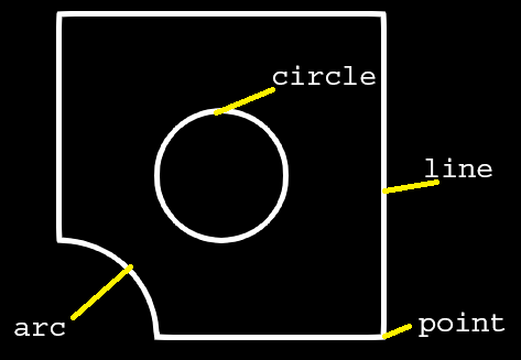
'circle':list[] # circle line, counterclockwise count
# set
# [
# [R,[CX,CY,CZ],[A0, A1]] # arc_1
# ...
# ]
# A1 ^
# | /
# | /
# | R
# | /
# |/
# (i:CX,CY,CZ)------A0
# options
R:float() # circle radius
CX:float() # point i center x coord.
CY:float() # point i center y coord.
CZ:float() # point i center z coord.
A0:str(e.g. val.='0') # angle begin [rad]
A1:str(e.g. val.='Pi/2') # angle end [rad]
#-----------------------
# example:
#-----------------------
# circle = [[30, [100, 100, 0], ['0', '2*Pi']]
# circles have priority numbering over arcs; pay attention to the plane numbering.
# see the generated model (.geo) in gmsh for correct setting
'arc': list[] # arc 3 points needed
# set
# [
# [point_i_begin:int, point_j_midle:int, , point_k_end:int]
# ...
# ]
#-----------------------
# example:
#-----------------------
# points = [
# [0, 0, 0], # ponto 1
# [200, 0, 0], # ponto 2
# [200, 40, 0], # ponto 3
# [100, 40, 0], # ponto 4
# [90, 30, 0], # ponto 5
# [0, 30, 0], # ponto 6
# [90, 40, 0], # ponto 7
# ]
# lines = [
# [1, 2], # linha 1
# [2, 3], # linha 2
# [3, 4], # linha 3
# [5, 6], # linha 4
# [6, 1], # linha 5
# ]
# arcs = [
# [5, 7, 4], # arco, adiciona uma nova linha 6
# ]
# plane = [
# [1, 2, 3, 6, 4, 5], # plane 1, sequencia das linhas
# ]
# You can add a list of lines to form a plan.
# To remove a plan within another, add the "-" symbol to the number.
# If the same number is followed by another sequence with a positive value,
# the program will remove and add a plan, creating a new material.
'planelist': list[] # planes lines conec., counterclockwise count
# set
# [
# [line_1_plane_1:int, ..., line_n_plane_1:int]
# ...
# ]
# (l)-----{3}-----(k)
# | |
# | |
# {4} [1] {2}
# | |
# | |
# (i)-----{1}-----(j)
#-----------------------
# example:
#-----------------------
# plane = [[1, 2, 3, 4]] add a new plane with the lines 1, 2, 3, 4
# plane = [[1, 2, 3, 4], [-5]] remove the line 5 ('circle') from the main plane with the lines 1, 2, 3, 4
# plane = [[1, 2, 3, 4], [-5], [5]] remove the line 5 ('circle') and add a new plane 5 ('circle') from the main plane with the lines 1, 2, 3, 4
'meshconfig':dict{} # mesh configuration inputs
# options
'mesh': str() # !!! mandatory option !!! set a type of mesh used in analysis
'sizeelement':float() # size min. of elements
'numbernodes':int() # select a number of nodes in line, only to 'line2/ line3' >see: Table 2 - Mesh List to more informations
'extrude':float() # extrude dimensional, in z diretion, from a xy plane
'meshmap':dict{} # gen. a mapped structured mesh
# option
'on': bool() # turn on(true/ false)
True
False
'edge': [ # select edge(lines) to map (only in 'on':True)
'all'
or
TAGS NUMB:list[int()] # select all edge or a specific edge
]
'numbernodes':list[int()] # select a number of nodes in each edge
#-----------------------
# example:
#-----------------------
# 'meshmap': {'on': True,
# 'edge': [[1, 2, 3], [4, 5, 6, 7]] or 'all',
# "numbernodes": [12, 8],
# [ adv ]
# Developed a robust Gmsh script that reorders nodes based on spatial coordinates (Z-Y-X)
# while preserving all physical groups and entity metadata for optimized FEM assembly.
# It is not compatible with 'meshmap'.
'reordermesh': bool() # turn on(true/ false)
True
False
# ==============================================================================
# Finally, pass the modeldata to the Model constructor API with the configured data and commands.
# ==============================================================================
fea.Model(modeldata)
Physics Setting
# ==============================================================================
# physicdata is a Python dictionary that contains the commands for physics set
# ==============================================================================
physicdata = dict()
# ==============================================================================
# physic set
# ==============================================================================
physicdata["PHYSIC"] = dict()
Domain
# ==============================================================================
# set the domain
# ==============================================================================
physicdata["PHYSIC"]["DOMAIN"]: str()
      # options
      'structural'
      'thermal'

      # [dev]
      'fluid'
Loads
# ==============================================================================
# configuration of loads applied to physics
# ==============================================================================
physicdata["PHYSIC"]["LOAD"] = list[load_set_1:dict(),..., load_set_n:dict()]
keys
"TYPE":str() 		          # type force n def.
      # options
      'forcenode'					# force in nodes, concentrated load
      'forceedge'					# force in edge, distributed load
      'forcesurf'					# force in surface, distributed load
      'forcebeam'					# force in beam only opt., distributed load

      # [adv]
      'forcebody'
      'strainzero'

      # heat options
      'heatfluxedge'
      'heatfluxsurf'
      'convectionedge'
      'convectionsurf'
      'heatgeneration'

"DOF":str()				          # dof direction of force n
      # options
      'fx'						      # force in x dir.
      'fy'						      # force in y dir.
      'fz'						      # force in z dir.
      'pressure'            # pressure app. in normal direction
      'tx'						      # torque/moment in x dir.
      'ty'						      # torque/moment in y dir.
      'tz'						      # torque/moment in z dir.
      'masspoint'					  # mass concentrated applied in node/point
      'spring2ground'				# spring connected node to ground/fixed end
      'damper2ground'				# damper connected node to ground/fixed end

# ----- OPT. WITH LOC SEEKERS
"DIR":str()				          # set direction >see: Axis Diretions
      # options
      'node'						    # node in mesh
      'lengthx'					    # length line in x dir., beam only option [legacy version]
      'lengthy'					    # length line in y dir., beam only option [legacy version]
      'lengthz'					    # length line in z dir., beam only option [legacy version]
      'edgex'						    # edge def in x dir. >'LOC': {'x':float(coord. x nodes), 'y':999(select all node in y dir.), 'z':float(coord. z nodes)}
      'edgey'						    # edge def in y dir.
      'edgez'						    # edge def in z dir.
      'surfxy'					    # surf def in xy plane >'LOC': {'x':999, 'y': 999, 'z':float(coord. z nodes)}
      'surfyz'					    # surf def in yz plane
      'surfzx'					    # surf def in zx plane

"LOC":dict()				        # coord. node locator >see: Axis Diretions
      'x':float()				    # x coord. node
      'y':float()				    # y coord. node
      'z':float()           # z coord. node

# ----- OPT. WITH TAG SEEKERS
"DIR":str()				          # set direction >see: Axis Diretions
      # options
      'point'						    # point number in tag list
      'edge'						    # edge number in tag list
      'surf'						    # surface number in tag list

"TAG":int()					        # tag number of regions type, used with gmsh mesh gen, view list

#  look up the corresponding node number in the Paraview, and add 1.
#  For example: node_paraview = 0 --> 0 + 1 --> MESHNODE = [1]
"MESHNODE": list[int()]     # select the node ([1]) or nodes list([1, 2, 3, ...]) number directly from the mesh

"VAL":list()				        # value list of force on steps, signal +/- is the direction
Boundary Conditions
# ==============================================================================
# configuration of boundary conditions applied to physics
# ==============================================================================
physicdata["PHYSIC"]["BOUNDCOND"] = list[bc_set_1:dict(),..., bc_set_n:dict()]
keys
"TYPE":str() 		            # type force n def.
      # options
      'fixed'							  # fixed boundary condition u=0. More in
      'displ'							  # displ boundary condition u!=0.

      # [adv]
      'cycsym'
      'bloch'

      # heat options
      'insulated'
      'temperature'

"DOF":str()			            # dof direction of force n
      # options
      'ux'							    # displ in x dir.
      'uy'							    # displ in y dir.
      'uz'							    # displ in z dir.
      'rx'							    # rotation in x dir.
      'ry'							    # rotation in y dir.
      'rz'							    # rotation in z dir.
      'full'							  # full dof

# ----- OPT. WITH LOC SEEKERS
"DIR":str()				          # set direction >see: Axis Diretions
      # options
      'node'							  # node in mesh
      'edgex'							  # edge def in x dir. >'LOC': {'x':float(coord. x nodes), 'y':999(select all node in y dir.), 'z':float(coord. z nodes)}
      'edgey'							  # edge def in y dir.
      'edgez'							  # edge def in z dir.
      'surfxy'						  # surf def in xy plane >'LOC': {'x':999, 'y': 999, 'z':float(coord. z nodes)}
      'surfyz'						  # surf def in yz plane
      'surfzx'						  # surf def in zx plane

"LOC":dict()
      # options					    # coord. node locator >see: Axis Diretions
      'x':float()				    # x coord. node
      'y':float()				    # y coord. node
      'z':float()           # z coord. node

# ----- OPT. WITH TAG SEEKERS
"DIR":str()				          # set direction >see: Axis Diretions
      # options
      'point'							  # point number in tag list
      'edge'							  # edge number in tag list
      'surf'							  # surface number in tag list

"TAG":int()					        # tag number of regions type, used with gmsh mesh gen, view list

#  look up the corresponding node number in the Paraview, and add 1.
#  For example: node_paraview = 0 --> 0 + 1 --> MESHNODE = [1]
"MESHNODE": list[int()]     # select the node ([1]) or nodes list([1, 2, 3, ...]) number directly from the mesh

"VAL":list()				        # value list of dislp on steps
Coupling
# ==============================================================================
# configuration of coupling applied to physics
# ==============================================================================
physicdata["COUPLING"] = dict()
keys
"TYPE":
      # options
      'thermalstress',       # CouplSolver

      # [dev]
      'fsi'

# To perform a coupled analysis, the same model is used, and the post-processing
# data from the first simulation is passed as input to the coupled simulation.
"POST": [PostProcessData]   # post-processing data from the previous simulation
#                          myfempy solver blackbox structure
#                               Fist Simulation [1]

# input                                API                 outputs

# Model [1]                      +---------------+
# BounCond + Loads [1]   -->     | FistSolver    |  -->    PostProcessData [1]
# SolverSet [1]                  +---------------+


#                               Coupled Simulation [2]

# input                                API                 outputs

# Model [1]                     +---------------+
# BounCond + Loads [2]  -->     | CouplSolver   |  -->     PostProcessData [2]
# PostProcessData [1]           +---------------+
# SolverSet [2]
# ==============================================================================
# Finally, pass the physicdata to the Physic constructor API with the configured data and commands
# ==============================================================================
fea.Physic(physicdata)
Preview analysis
# ==============================================================================
# Preview set
# ==============================================================================
previewset = {'RENDER':
{
'filename': str(),

'show': bool()
# options
    True
    False

'scale': int(),

'savepng': bool(),
# options
    True
    False

'lines': bool(),   # wireframe lines
# options
    True
    False

'plottags': {
# options
    'point': True/ False
    'line':  True/ False
    'surf':  True/ False
}

# beam cross-section view optinos
'cs': True,
},
}
fea.PreviewAnalysis(previewset)
Solver Set
# ==============================================================================
# solver set
# ==============================================================================
solverset = {"STEPSET":
{
'type': str()
    # options
    'table',      # tabulated values, e.g. [step0, step1, ..., stepN]
    'mode',       # vibration modes
    'freq',       # frequency scale, np.linspace
    'time',       # time scale, np.linspace
'start': int(),
'end': int(),
'step': int(),
    },

'SYMM': bool(),   # matrix symmetric assembler
# options
    True
    False

# [ adv ]
'IBZ': np.array(  # Brillouin zone
  [[0.0, 0.0],    # O
   [np.pi, 0.0],  # A
   [np.pi, np.pi],# B
   [0.0, 0.0]]),  # O

#             (B)
#             /^
#            / |
#           /  |
#          /   |
#         /    |
#        /     |
#      </      |
#      (O)--->(A)

# [ dev ]
'MP': bool(),     # multi processing
# options
    True
    False
}
solverdata = fea.Solve(solverset)
Post-Process
# ==============================================================================
# post-process set
# ==============================================================================
postprocset = {
"SOLVERDATA": solverdata,

"COMPUTER": {
'structural': {
    'displ': True/ False,
    'stress': True/ False}

'thermal': {
    'temp': True/ False,
    'heatflux': True/ False}

# [dev]
'fluid',
},

"PLOTSET": {
'show': True/ False,
'filename': str(),
'savepng': True/ False},

"OUTPUT": {
'log': True/ False,
'get':{
    'nelem': True/ False,     # number of elements in the mesh
    'nnode': True/ False,     # number of nodes in the mesh
    'inci': True/ False,      # list of elements
    'coord':True/ False,      # list of nodes coodinate
    'tabmat':True/ False,     # list of material property
    'tabgeo':True/ False,     # list of geometry property
    'bc_list':True/ False,    # list of constraints (boundary conditions)
    'lo_list':True/ False,    # list of loads
    'u_list':True/ False,     # list of solutions
    'numpy_decimals': int(),  # decimals to print, e.g. 8
}
}}
postprocdata = fea.PostProcess(postprocset)
Tutorials
The main objective of these tutorials is to help the user explore the various modeling and simulation options that the project allows.
This tutorial was developed during the initial implementation of the project; therefore, the information contained herein is not 100% up-to-date with the latest version of myfempy. See the API documentation for a more modern version.
Mesh
Manual Mesh
--8<-- "docs/tutoriais/malha/manual_mesh_gen.py"
Legacy Mesh
--8<-- "docs/tutoriais/malha/legacy_mesh_gen.py"
GMSH Mesh Basic
--8<-- "docs/tutoriais/malha/gmsh_basic_comm.py"
GMSH Mesh Advanced
--8<-- "docs/tutoriais/malha/gmsh_adv_comm.py"
GMSH Mesh Solids
--8<-- "docs/tutoriais/malha/gmsh_solid_comm.py"
GMSH Mesh Importing CAD models (.stp/.step)
--8<-- "docs/tutoriais/malha/gmsh_cad_comm.py"
GMSH Mesh Importing mesh files (.msh2)
--8<-- "docs/tutoriais/malha/gmsh_msh2_comm.py"
Simulations
Structural Static
--8<-- "docs/tutoriais/analise_pos/set_strucutural_model.py"
Structural Static Solid Gmsh API
--8<-- "docs/tutoriais/analise_pos/set_gmsh_api_model.py"
Structural Vibration
--8<-- "docs/tutoriais/analise_pos/vibration_struct.py"
Heat
--8<-- "docs/tutoriais/analise_pos/set_heat_model.py"
Thermo Mechanical Coupling
--8<-- "docs/tutoriais/analise_pos/tmc.py"
SET NEW MATERIAL: ORTHOTROPIC ELASTIC
SET NEW MATERIAL ORTHOTROPIC ELASTIC
--8<-- "docs/tutoriais/material/set_user_material.py"
Appendix
Useful Links
GMSH FreeCAD Python NumPy SciPy Computer-aided design Finite element method Young’s modulus Poisson’s ratio Shear modulus Density List of moments of inertia Boundary value problem Gaussian quadrature International System of Units
Axis Diretions
# 		 |
# 		 [Y]
# 		 |		P1 -- principal plane
# 		 |		P2 -- secondary plane
# 		 |__edgey__
# 	    /|		   |
# 	   / |   P1    |
# 	  /	 | surfxy  edgex
# 	 /  f|		   |
#   /  r |_________|____________[X]__
#  | u  /          /
#  |s z/   P2     /
#  | y/	 surfzx  edgez
#  | /          /
#  |/__________/
#  /
# [Z]
#/
Cross Section Dimensions
Geometric Cross-Section Libraries
# 						:
# 						[Y]
# 						:
#  ___		 ___________:___________
# 	| 		|_______    :    _______|
# 	|				|	:	|
# 	|			 -->|	:	|<-------------(t)
# 	|				|	:	|
# 	|				|	:	|
# 	|				|	:	|
#   (h)				|  (CG).|..........[Z]..
# 	|				|		|
# 	|				|		|
# 	|				|		|
# 	|				|		|
# 	|		 _______|		|_______	___
#  _|_		|_______________________|  	_|_(d)


# 			|-----------(b)---------|
Table 1 - Elements List
| element | id | description |
|---|---|---|
| block | 11 | Spring + Mass 1D-space 1-node_dofs |
| structbeam | 16 | Beam Structural Element 1D-space 6-node_dofs |
| structplane | 22 | Plane Structural Element 2D-space 2-node_dofs |
| structsolid | 33 | Solid Structural Element 3D-space 3-node_dofs |
| heatplane | 21 | Plane Heat Element 2D-space 1-node_dof |
| heatsolid | 31 | Solid Heat Element 3D-space 1-node_dofs |
Table 2 - Shape (Mesh) List
| mesh | id | description | Gauss Points Opt. |
|---|---|---|---|
| line2 | 21 | Line 2-Node Shape 2-nodes_conec 1-interpol_order | 1/ 2/ 4/ 8 |
| line3 | 32 | Line 3-Node Shape 3-nodes_conec 2-interpol_order | 1/ 2/ 4/ 8 |
| tria3 | 31 | Triangular 3-Node Shape 3-nodes_conec 1-interpol_order | 1/ 3/ 7 |
| tria6 | 62 | Triangular 6-Node Shape 6-nodes_conec 2-interpol_order | 1/ 3/ 7 |
| quad4 | 41 | Quadrilateral 4-Node Shape 4-nodes_conec 1-interpol_orde | 1/ 2/ 3/ 4/ 8/ 9 |
| quad8 | 82 | Quadrilateral 8-Node Shape 8-nodes_conec 2-interpol_order | 1/ 2/ 3/ 4/ 8/ 9 |
| hexa8 | 81 | Hexaedron 8-Node Shape 8-nodes_conec 1-interpol_order | 1/ 2/ 3/ 4/ 8/ 9 |
| tetr4 | 41 | Tetrahedron 4-Node Shape 4-nodes_conec 1-interpol_orde | 1/ 3/ 5 |
Table 3 - Solvers List
| solver | id | description | mandatory parameters | optional parameters |
|---|---|---|---|---|
| SteadyStateLinear | Steady State Linear Solver Class (Static Linear) | Model, Assembly: [stiffness, loads], ConstrainsDof: [freedof, constdof] | Assembly: [bcdirnh], Solverset: [nsteps] | |
| SteadyStateLinearIterative | Steady State Linear Iterative Solver Class (Static Linear) | Model, Assembly: [stiffness, loads], ConstrainsDof: [freedof, constdof] | Assembly: [bcdirnh], Solverset: [nsteps, tol, maxiter] | |
| DynamicEigenLinear | Dynamic Eigen (modal problem) Linear Solver Class | Model, Assembly: [stiffness, mass], ConstrainsDof: [freedof] | Solverset: [modeEnd:nsteps] | |
| DynamicHarmonicResponseLinear | Dynamic Harmonic Response Forced System Steady State Linear Solver Clas | Model, Assembly: [stiffness, mass, loads], ConstrainsDof: [freedof] | Solverset: [freqStart:start, freqEnd:end,freqStep:nsteps] | |
| dev TransientLinear | ||||
| adv StaticLinearCyclicSymmPlane | Static Linear Cyclic Symmetry Plane Solver Class | Model, Physic, Assembly: [stiffness, loads], ConstrainsDof: [freedof, fixedof(leftdof, rightdof, interdof)*] | Solverset: [nsteps] | |
| adv HomogenizationPlane | Homogenization Plane Solver Class | Model, Assembly: [stiffness, loads], ConstrainsDof: [freedof, fixedof(strain)*] | ||
| adv PhononicCrystalInPlane | Phononic Crystal In-Plane Solver Class | Model, Assembly: [stiffness, mass], ConstrainsDof: [freedof, constdof(bloch)*] | Solverset: [nsteps, IBZ*] | |
| dev TopologyOptimization | ||||
*Note: See Solver Set
Legends
Table 4 - Material List
| material | id | description |
|---|---|---|
| UniAxialStress | Uni-Axial Stress Isotropic Material Class | |
| PlaneStress | Plane Stress Isotropic Material Class | |
| PlaneStrain | Plane Strain Isotropic Material Class | |
| SolidElastic | Solid Stress Isotropic Material Class | |
| HeatPlane | Heat Plane Isotropic Material Class | |
| HeatSolid | Heat Solid Isotropic Material Class | |
| UserNewMaterial | User Defined Material API | |
Table 5 - Consistent Units
| Quantity | SI(m) | SI(mm) |
|---|---|---|
| length | m | mm |
| mass | kg | tonne |
| time | s | s |
| temperature | °C | °C |
| rotation | rad | rad |
| acceleration/ gravity | m/s^2 | mm/s^2 |
| density | kg/m^3 | tonne/mm^3 |
| force | N(kg⋅m⋅s^−2) | N |
| moment | N-m | N-mm |
| frequency | Hz(s^-1) = (rad/s)/(2.pi) | Hz |
| pressure/ stress | Pa(N/m^2) | MPa(N/mm^2) |
| energy | J(kg⋅m^2⋅s^−2) | mJ(tonne⋅mm^2⋅s^−2) |
| power | W(kg⋅m^2⋅s^-3) | mW(tonne⋅mm^2⋅s^-3) |
| thermal conductivity | W/(m.°C) | mW/(mm·°C) |
| thermal expansion | (m/m)/°C | (mm/mm)/°C |
| heat flux | W/m^2 | W/mm^2 |
| viscosity | Pa.s | MPa.s |
See International System of Units